Comparethemarket.com is exploring ways to offer a more personalised, relevant experience to each of its customers. In order to achieve a great content recommendation and targeted products, it is strongly advised to model BGL’s user data to better understand customer’s behaviour.
For the purpose of this case study, a sample dataset was kindly provided by BGL to assist in the process. RStudio is the software that is used with the modelling of the data being implemented using Machine Learning techniques.
Context and Proposed Approach
As Bryan Eisenberg once said, “Our jobs as marketers are to understand how the customer wants to buy and help them to do so.” Having that in mind, one invaluable question for every business to answer, is “Would someone buy this product?” or better yet, “How probable would be that someone would buy that product?”. The answer to these questions can be achieved with the assistive power of predictive modelling. And this is where data comes into play.
Using Logistic Regression with L1 penalisation (Lasso Logistic Regression), we intend to build a recommendation model that will have a specific probability as an output. This probability indicates how probable would be that a specific user would interact with the respective product. For instance, if the output of the model is “1”, this suggests that the data yields a high confidence that the customer would interact with the product, whereas an output of “0” suggests otherwise. The reason for the choice of this particular machine learning model is due to the fact that Logistic Regression is a powerful model for such occasions.
Preliminary Insights and Conclusions
## REQUIRED PACKAGES
library(ggplot2)
library(dplyr)
library(ROCR)
library(caret)
library(randomForest)
library(glmnet)
library(gridExtra)
In order to have the best results possible, it is highly important to explore the data and prepare it for modelling - preprocessing.
First, let us explore how the data looks like
## READ THE DATA
data <- read.csv("CTM_DataScientistCaseStudy.csv")

## EXPLORE HOW THE DATA LOOKS
dim(data)  ## 100.000   6
## [1] 100000 6
head(data)
##   UserID Age UserSegment  Recency PriorEvent Event
## 1      1  56           A Inactive          0     0
## 2      2  39           A Inactive          0     0
## 3      3  62           A   Active          1     1
## 4      4  29           C Inactive          0     0
## 5      5  41           C  Dormant          0     0
## 6      6  53           A   Active          1     1
tail(data)
##        UserID Age UserSegment Recency PriorEvent Event
## 99995   99995  23           C  Active          0     0
## 99996   99996  43           C  Active          0     0
## 99997   99997  58           C  Active          0     0
## 99998   99998  70           A  Active          0     0
## 99999   99999  24           C  Active          0     0
## 100000 100000  45           C  Active          0     0
The data consists of 100.000 instances (i.e. customers) and 6 columns that correspond to
## EXPLORE THE ATTRIBUTES OF THE DATA
colnames(data)
## [1] "UserID"      "Age"         "UserSegment" "Recency"     "PriorEvent"
## [6] "Event"
We observe that there are no duplicated entries in the data and that every user ID is unique and corresponds to a single individual.
## CHECK FOR DUPLICATED ENTRIES
sum(duplicated(data))    ## 0 DUPLICATED
## [1] 0
n_distinct(data$UserID) ## 100.000 UNIQUE CUSTOMER IDS
## [1] 100000
For a sanity check, we make sure that the columns of the data are in the correct format as this plays a major role in the modelling process later on.
## CHECK IF VARIABLES ARE IN THE CORRECT FORM
str(data)
## 'data.frame':    100000 obs. of  6 variables:
##  $ UserID     : int  1 2 3 4 5 6 7 8 9 10 ...
##  $ Age        : int  56 39 62 29 41 53 30 44 71 40 ...
##  $ UserSegment: Factor w/ 4 levels "A","B","C","NULL": 1 1 1 3 3 1 3 1 3 2 ...
##  $ Recency    : Factor w/ 4 levels "Active","Dormant",..: 3 3 1 3 2 1 3 1 2 1 ...
##  $ PriorEvent : int  0 0 1 0 0 1 0 0 0 0 ...
##  $ Event      : int  0 0 1 0 0 1 1 0 0 1 ...
To explore the data even further, it is highly recommended to have a summary of the data and the values that exist in each column. We also investigate for any N/A values. As it is shown below,
## TAKE A GENERAL INSIGHT OF THE DATA
summary(data)
##      UserID            Age        UserSegment      Recency
##  Min.   :     1   Min.   :18.00   A   :21017   Active  :55428
##  1st Qu.: 25001   1st Qu.:28.00   B   :19973   Dormant :22275
##  Median : 50000   Median :36.00   C   :58517   Inactive:21804
##  Mean   : 50000   Mean   :38.75   NULL:  493   NULL    :  493
##  3rd Qu.: 75000   3rd Qu.:48.00
##  Max.   :100000   Max.   :75.00
##    PriorEvent          Event
##  Min.   :0.00000   Min.   :0.0
##  1st Qu.:0.00000   1st Qu.:0.0
##  Median :0.00000   Median :0.0
##  Mean   :0.09178   Mean   :0.3
##  3rd Qu.:0.00000   3rd Qu.:1.0
##  Max.   :1.00000   Max.   :1.0
cat("The number of N/A values are:", sum(is.na(data)), "\n") ## NO N/A VALUES
## The number of N/A values are: 0
cat("The valid User Segment entries are:", levels(data$UserSegment), "\n") ## "A" "B" "C" "NULL"
## The valid User Segment entries are: A B C NULL
cat("The valid Recency entries are:",levels(data$Recency)) ## "Active" "Dormant" "Inactive" "NULL"
## The valid Recency entries are: Active Dormant Inactive NULL
Although there are no N/A values per se, we discovered entries both in the “UserSegment” and “Recency” columns with the entry of “NULL”. These entries are 493 in both cases, which corresponds to almost 0.5% of the data. Therefore, and since we do not have any data on what the NULL values mean, we are going to ignore these records as this approach is considered an effective method for handling such data when the number of the occurrences is so low.
Our predictions will be focused on the “Event” variable as it will be treated as our response. “Event” will have the value of “1” when a customer interacted with a specific product or service (i.e. shown interest) and the value “0” otherwise. In our sample, 70% percent of the data corresponds to products where the customer showed no interest and the rest of 30% the opposite.
## DISTRIBUTION OF THE INTEREST OF THE CUSTOMER FOR A PRODUCT
table(data$Event)        ## POSTERIOR: NO INTEREST(0): 70.000      INTEREST(1): 30.000
##     0     1
## 70000 30000
Apart from that, previous knowledge of the customer’s interest is also available in the “PriorEvent” variable where we see that the percentages are slightly more skewed in favor of the “No Interest” incidents. More specifically, almost 90% of the proposed products, were of no interest to the customers.
## DISTRIBUTION OF THE PRIOR INTEREST OF THE CUSTOMER FOR A PRODUCT
table(data$PriorEvent)   ## PRIOR: NO INTEREST(0): 90.822      INTEREST(1): 9.178
##     0     1
## 90822  9178
Two major observations need to be discussed here. The first one is about what changed between the period of the “PriorEvent” and the “Event”. Whether this corresponds to a change in a marketing campaign or a period of economic growth, it could be a factor that needs to be investigated in order to understand the difference of interest of the customers. The second point that needs to be discussed is the question that the BGL group is trying to answer out of the data. The variable “PriorEvent” is going to be part of the modelling process. This denotes that the output of the model will indicate the probability that a customer will re-grow, or not, interest in the particular product. Thus, the question that will be answered is going to be whether the customer will re-perform an action to this particular product.
PRELIMINARY ANALYSIS
Our age range is from customers between 18 and 75 years old with an average age of almost 39 years old.
summary(data$Age) ## CHECK THE SUMMARY OF THE AGE
##    Min. 1st Qu.  Median    Mean 3rd Qu.    Max.
##   18.00   28.00   36.00   38.75   48.00   75.00
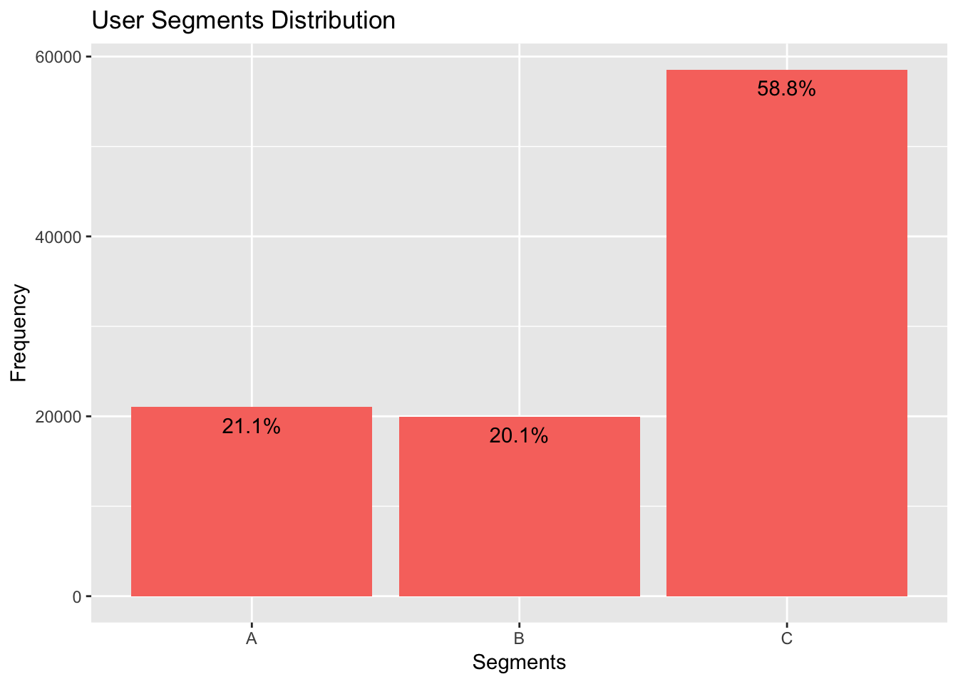
The major user segment is the “C” segment which accounts for 58,8% of the data and the rest almost evenly split between segments “A” and “B”; Segment “A” with 21,1% and segment “B” with 20,1%.
## DISTRIBUTION OF SEGMENTS
Segment <- as.data.frame(table(data$UserSegment))
Segment <- Segment[Segment$Var1 != "NULL",]   ## REMOVE THE NULL OBSERVATIONS
ggplot(data = Segment, aes(x = Var1, y = Freq)) +
  geom_bar(stat = "identity", fill = "#F8766D") +
  geom_text(y = Segment[,2] - 2000,
            aes(label = paste0(round((Segment[,2]/sum(Segment[,2]))*100, digits = 1), "%" ))
  ) +
  labs(x = "Segments", y = "Frequency") +
  ggtitle("User Segments Distribution")
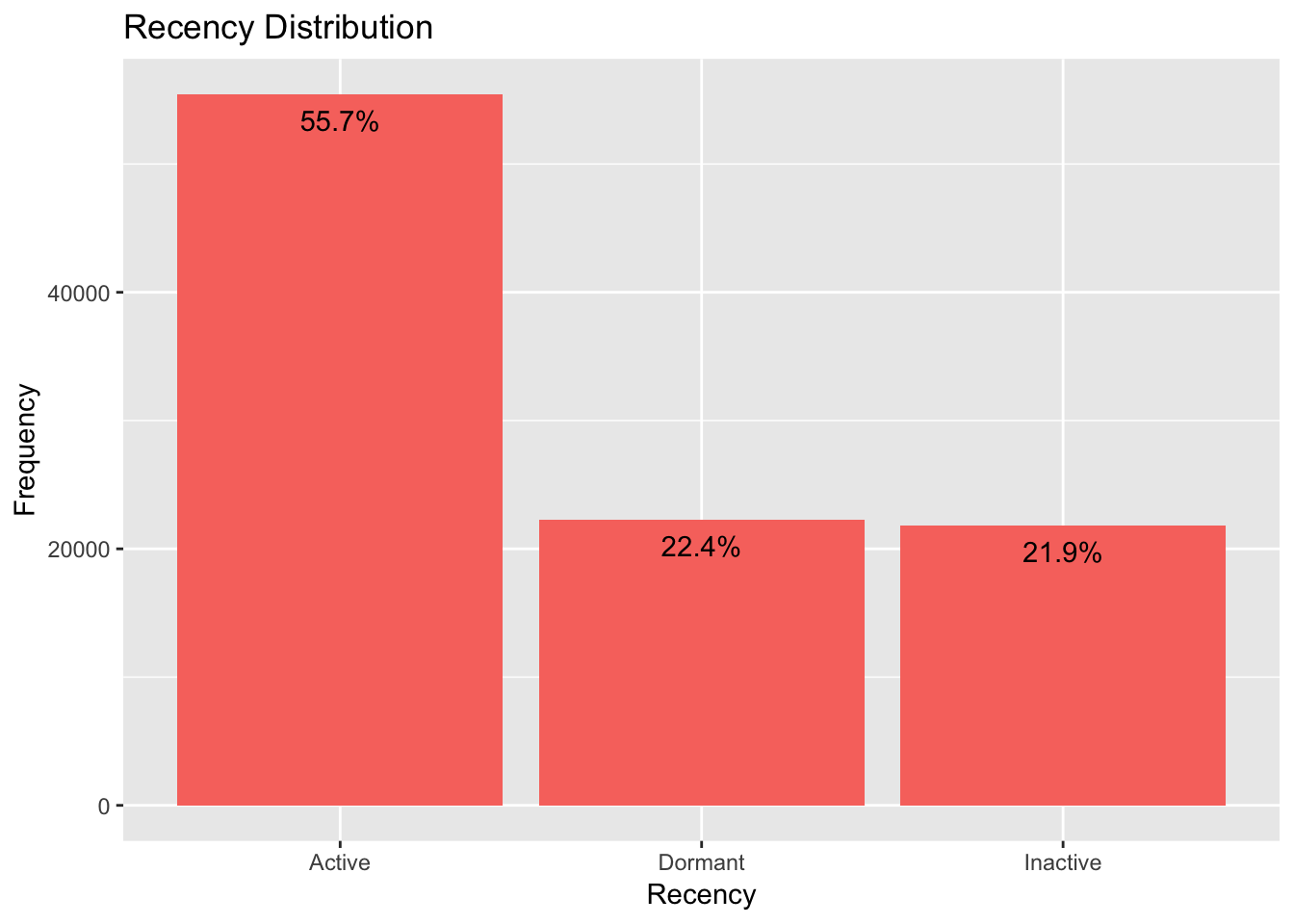
In addition, almost 55,7% of the data are described as “Active” users, 22,4% as “Dormant” and 21,9% as “Inactive”.
## DISTRIBUTION OF RECENCY
RecencyDis <- as.data.frame(table(data$Recency))
RecencyDis <- RecencyDis[RecencyDis$Var1 != "NULL", ]  ## REMOVE THE NULL OBSERVATIONS
ggplot(data = RecencyDis, aes(x = Var1, y = Freq)) +
  geom_bar(stat = "identity", position = "dodge", fill = "#F8766D") +
  geom_text(y = RecencyDis[,2] - 2000,
            aes(label = paste0(round((RecencyDis[,2]/sum(RecencyDis[,2]))*100, digits = 1), "%" ))
            ) +
  labs(x = "Recency", y = "Frequency") +
  ggtitle("Recency Distribution")
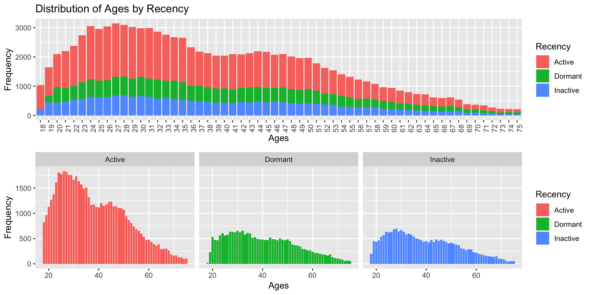
We also observe that the “Ages” distribution with respect to the “Recency” status follows the same pattern. The age group of 20-35 looks to be the most frequent in the respective “Recency” statuses.
## DISTRIBUTION OF THE AGES ACCORDING TO RECENCY
## VISUALISE THE CORRESPONDING DATA
AgeActivity <- as.data.frame(data %>%
       group_by(Recency, Age)
     %>% summarise(counts = n())
     %>% filter(Recency != "NULL")
     %>% arrange(desc(counts))
)

p1 <- ggplot(data = AgeActivity, aes(x = factor(AgeActivity[,2]), y = AgeActivity[,3])) +
  geom_bar(stat = "identity", aes(fill = AgeActivity[,1])) +
  labs(x="Ages", y="Frequency", fill="Recency") +
  ggtitle("Distribution of Ages by Recency") +
  theme(axis.text.x = element_text(angle = 90, hjust = 1))

p2 <- ggplot(data = AgeActivity, aes(x = AgeActivity[,2], y = AgeActivity[,3], fill = AgeActivity[,1])) +
  geom_bar(stat = "identity") +
  facet_grid(AgeActivity[,1]) +
  labs(x="Ages", y="Frequency", fill="Recency")

grid.arrange(p1, p2, ncol = 1)
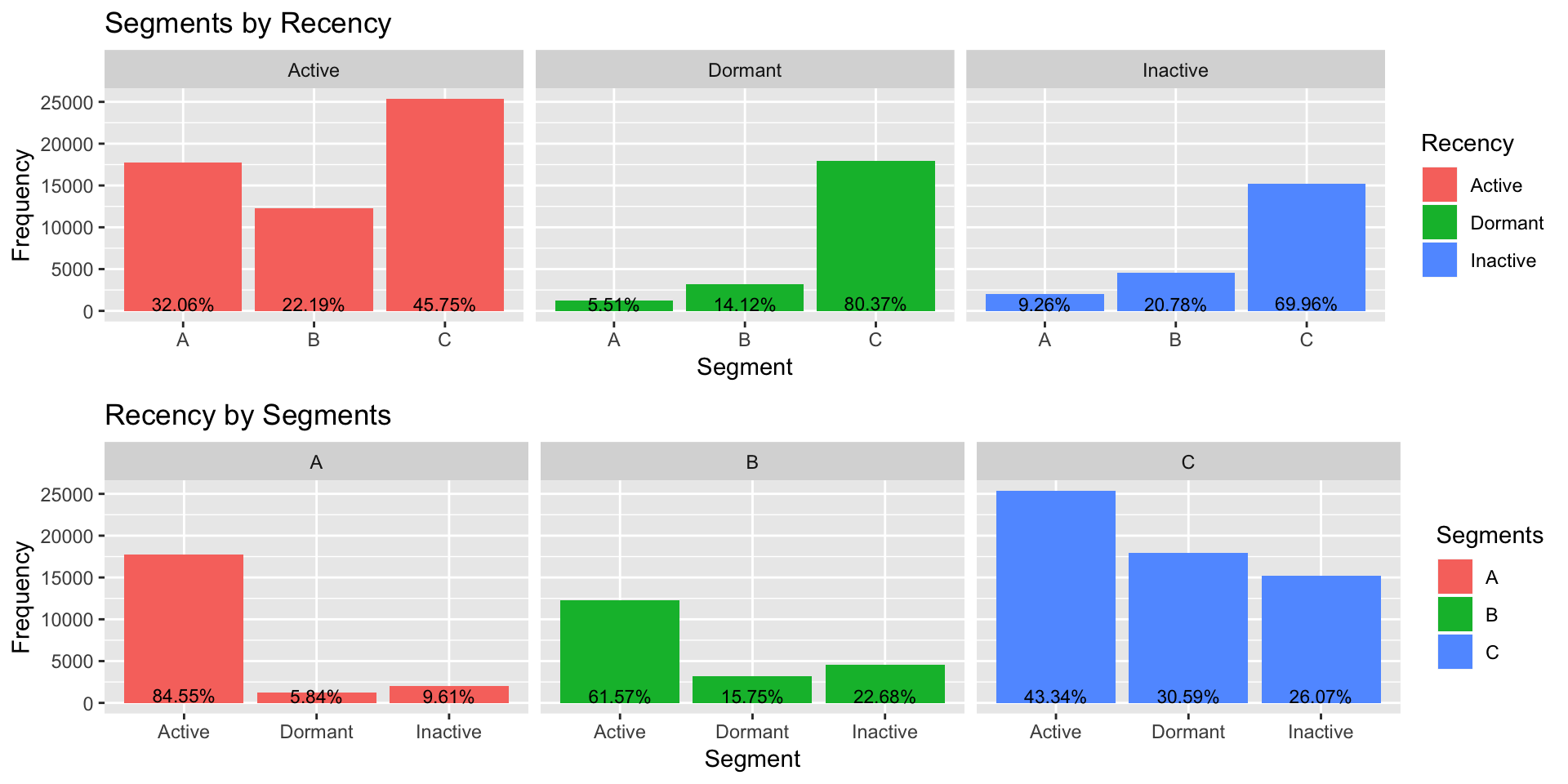
Finally, for the different types of “Recency” and “Segments”, we can see how the Users are distributed in the graphs below.
## DISTRIBUTION OF THE RECENCY ACCORDING TO USER SEGMENT
## VISUALISE THE CORRESPONDING DATA
ActivitySegment <- as.data.frame(data %>%
                                   group_by(Recency, UserSegment)
                                 %>% summarise(counts = n())
                                 %>% filter(Recency != "NULL")
                                 %>% arrange(desc(counts))
                                 %>% mutate(percent = round((counts/sum(counts))*100, digits = 2))
)

p1.2 <- ggplot(data = ActivitySegment, aes(x = ActivitySegment[,2], y = ActivitySegment[,3], fill = ActivitySegment[,1])) +
  geom_bar(stat = "identity", position = "dodge") +
  geom_text(size = 3, stat = "identity", position = position_dodge(.9), aes(y = ActivitySegment[,4]+ 800, label = paste0(ActivitySegment[,4], "%") )) +
  facet_grid(ActivitySegment[,1]) +
  labs(x = "Segment", y = "Frequency", fill = "Recency") +
  ggtitle("Segments by Recency")

## DISTRIBUTION OF THE USER SEGMENT ACCORDING TO RECENCY
ActivitySegment2 <- as.data.frame(data %>%
                                   group_by(UserSegment, Recency)
                                 %>% summarise(counts = n())
                                 %>% filter(Recency != "NULL")
                                 %>% arrange(desc(counts))
                                 %>% mutate(percent = round((counts/sum(counts))*100, digits = 2))
)

p2.2 <- ggplot(data = ActivitySegment2, aes(x = ActivitySegment2[,2], y = ActivitySegment2[,3], fill = ActivitySegment2[,1])) +
  geom_bar(stat = "identity", position = "dodge") +
  geom_text(size = 3, stat = "identity", position = position_dodge(.9), aes(y = ActivitySegment2[,4] + 800, label = paste0(ActivitySegment2[,4], "%") )) +
  facet_grid(ActivitySegment2[,1]) +
  labs(x = "Segment", y = "Frequency", fill = "Segments") +
  ggtitle("Recency by Segments")

grid.arrange(p1.2, p2.2, nrow = 2)
MODEL CREATION AND CONCLUSIONS
Since there is a better understanding of the data, we can implement the Lasso Logistic Regression model to create our recommendation model. As it was mentioned, Lasso is an amazing technique as it prevents over-fitting by taking into account possible correlated features and eliminate variables that add noise to the model. Therefore, the final model is considered to provide with objective results and recommendations that can generalise well in unseen data.
In order for the model to work correctly, it is advised to be provided with balanced data; data that has the same number of Events = 1 and Events = 0. Since the proportion of our dataset is 70% in favor of products where the customer showed no interest, an artificially balanced dataset will be produced by undersampling the majority class. In other words, out of the 70,000 instances of Events = 0, a sample of 30,000 instances is going to be extracted to match the sample of 30,000 instances of Events = 1. Literature suggests undersampling in favor of techniques of oversampling. In addition, several iterations (e.g. 10 iterations) will be run in order to secure unbiased results due to sampling.
To validate the model, 10-Fold Cross Validation is performed and an additional test set is withheld from the training process with an 80%-20% split to test the model even further.
## SET NUMBER OF REPETITIONS
n <- 10
## EMPTY CONFUSION MATRIX TO BE STORED FROM VARIOUS REPETITIONS
confusion <- data.frame(r1 = rep(0,n), r2 = rep(0,n), r3 = rep(0,n), r4 = rep(0,n))

## AUC VALUE EMPTY VECTOR TO STORE AUC VALUES FROM VARIOUS REPETITIONS
auc.total <- vector(mode = "numeric", length = n)

## RUN THE MODEL
for(i in 1:n){
## CREATE BALANCED DATASET BY UNDERSAMPLING THE MAJORITY CLASS
event0 <- data[data$Event == 0,]
event0 <- sample_n(event0, 30000, replace = FALSE)  ## FROM MAJORITY CLASS, TAKE A 30.000 SAMPLE

event1 <- data[data$Event == 1,]    ## FROM MINORITY CLASS, TAKE ALL THE 30.000 INSTANCES
balancedData <- rbind(event0, event1)   ## CREATE THE BALANCED DATA

## TAKE THE DEISGN MATRIX
designMatrix <- sparse.model.matrix(Event ~ .  , data = balancedData[,-c(1)])[,-1]  ## REMOVE THE CUSTOMER ID AND THE INTERCEPT
response <- balancedData$Event  ## STORE THE RESPONSE VARIABLE

## SPLIT IN TRAIN AND TEST SET
ind <- sample(2, nrow(designMatrix), replace = TRUE, prob = c(0.8, 0.2))

trainData <- designMatrix[ind == 1,]
responseTrain <- response[ind == 1]
dim(trainData)

testData <- designMatrix[ind == 2,]
responseTest <- response[ind == 2]
dim(testData)

## CHECK FOR PROPORTION
# FOR DESIGN TRAIN
table(responseTrain)

# FOR DESIGN TEST
table(responseTest)

## LASSO CROSS VALIDATION TO FIND THE BEST LAMBDA
cv <- cv.glmnet(trainData, responseTrain,
                nfolds = 10,
                type.measure = "class",
                family = "binomial",
                alpha = 1)

## PREDICT ON TEST.SET (UNSEEN DATA) USING THE BEST LAMBDA FROM CROSS VALIDATION
predictions <- predict(cv, newx = testData, type = "response", s = "lambda.min")
pred.roc <- predictions     ## STORE THE PROBABILTIES FOR THE ROC CURVE TO BE USED LATER
cut_off <- 0.47             ## SELECT THE CUT-OFF TO CLASSIFY THE RESULT
predictions <- if_else(predictions >= cut_off, 1, 0)

## STORE AUC VALUE
predictions.bal <- prediction(pred.roc, responseTest)
auc <- performance(predictions.bal, "auc")
auc.total[i] <- unlist(slot(auc, "y.values"))

## STORE THE CONFUSION MATRIX FOR EVERY REPETITION
confusion[i,] <- as.vector(table(predictions, responseTest))
}
RESULTS
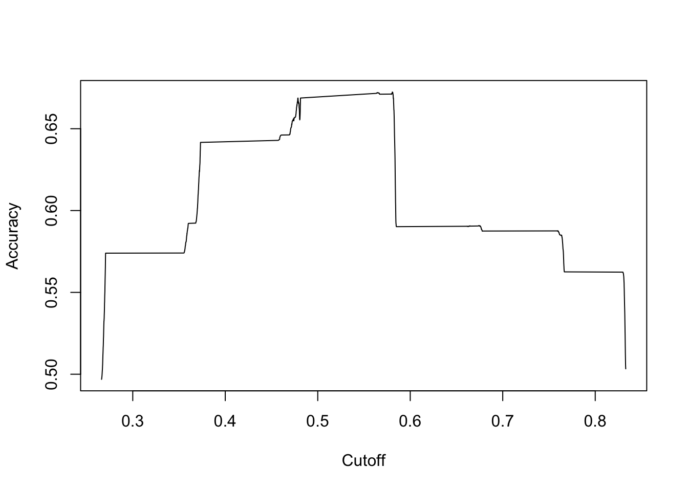
The most common and widest metric to rate the success of a machine learning model is the accuracy metric. As the name denotes, accuracy is the fraction of predictions the model got right in total. However, we are also interested in the proportion of the predictions that the user would interact with a product and the predictions that the user would not. Both of these proportions are measured with the Sensitivity and Specificity metrics respectively. Sometimes, we are more interested in obtaining a higher value in one of these metrics over the other as it is considered to be more important. In our case, more of a significant error it would be to not recommend a product that the customer would interact rather than suggesting a product that the customer would not. Therefore, a priority is to obtain a high value of Sensitivity as possible while keeping a reasonable balance between them. This can be achieved by being a little bit more willing to recommend a product to a customer. Recall that the model will have an output of a probability which means that an output of 0.5 would indicate half a chance of the customer re-showing interest for a particular product. Setting a cut-off slightly lower than that, we can be sure to not miss a high number of products or services that would be of an interest to a customer.
## CREATE A FUNCTION TO CALCULATE THE AVERAGE ACCURACY, SPECIFICITY, SENSITIVITY OF THE VARIOUS REPETITIONS
res <- function(x) {
  x <- matrix(as.numeric(x), ncol = 2)
  accur <- (x[1,1]+x[2,2])/sum(x)
  sens <- x[2,2]/sum(x[,2])
  spec <- x[1,1]/sum(x[,1])
  out <- list(Accuracy = accur, Specificity = spec, Sensitivity = sens)
  out
}
total <-  apply(confusion, 1, FUN = res)

## OBTAIN THE AVERAGE ACCURACY, SPECIFICITY, SENSITIVITY AND STANDARD DEVIATION OF THESE
avg.spec <-0
avg.acc <-0
avg.sens <- 0

spec.total <- vector(mode = "numeric", length = n)
sens.total <- vector(mode = "numeric", length = n)
acc.total <- vector(mode = "numeric", length = n)
for(i in 1:n){

  avg.acc = as.numeric(total[[i]][1]) + avg.acc
  acc.total[i] <- as.numeric(total[[i]][1])

  avg.sens = as.numeric(total[[i]][3]) + avg.sens
  sens.total[i] <- as.numeric(total[[i]][3])

  avg.spec = as.numeric(total[[i]][2]) + avg.spec
  spec.total[i] <- as.numeric(total[[i]][2])

}

## MODEL VALIDATION RESULTS
## AVERAGE AVERAGE ACCURACY, SPECIFICITY, SENSITIVITY
cat("The accuracy of the model for", n, "repetitions is:", round(avg.acc/n, digits = 2))
## The accuracy of the model for 10 repetitions is: 0.65
cat("The sensitivity of the model for", n, "repetitions is:", round(avg.sens/n, digits = 2))
## The sensitivity of the model for 10 repetitions is: 0.82
cat("The specificity of the model for", n, "repetitions is:", round(avg.spec/n, digits = 2))
## The specificity of the model for 10 repetitions is: 0.48
## STANDARD DEVIATIONS OF ACCURACY, SPECIFICITY, SENSITIVITY
cat("The standard deviation of the accuracy for", n, "repetitions is:", round(sd(acc.total),3))
## The standard deviation of the accuracy for 10 repetitions is: 0.007
cat("The standard deviation of the sensitivity for", n, "repetitions is:", round(sd(sens.total),3))
## The standard deviation of the sensitivity for 10 repetitions is: 0.03
cat("The standard deviation of the specificity for", n, "repetitions is:", round(sd(spec.total),3))
## The standard deviation of the specificity for 10 repetitions is: 0.043
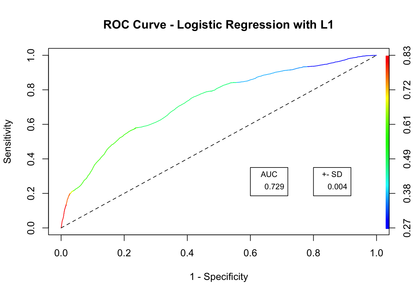
Last but not least, the following graphs create a bigger picture between the trade-off of Sensitivity and Specificity so as to have a wider sense of the performance of the machine learning model. The AUC value, which stands for Area Under the Curve, is another validation value that was put for cross-reference with the Accuracy, Sensitivity and Specificity.
## ROC CURVE
predictions.bal <- prediction(pred.roc, responseTest)
roc.lasso <- performance(predictions.bal, measure = "tpr", x.measure = "fpr")

## AUC
mean.auc <- round(mean(auc.total),3)   ## AVEGRAGE AUC
sd.auc <- round(sd(auc.total),3)       ## STANDARD DEVIATION AUC

## ACCURACY CUT-OFF
perf.bal.ac <- performance(predictions.bal, "acc")
plot(perf.bal.ac)
## PLOT ROC CURVE AND AUC VALUE TO FURTHER VALIDATE THE MODEL
plot(roc.lasso, colorize = TRUE, ylab = "Sensitivity", xlab = "1 - Specificity", main = "ROC Curve - Logistic Regression with L1")
lines(c(0,1), c(0,1), col = "black", lty = 2)
legend(.6, .35, mean.auc, title = "AUC", cex = .8)
legend(.8, .35, sd.auc, title = "+- SD", cex = .8)
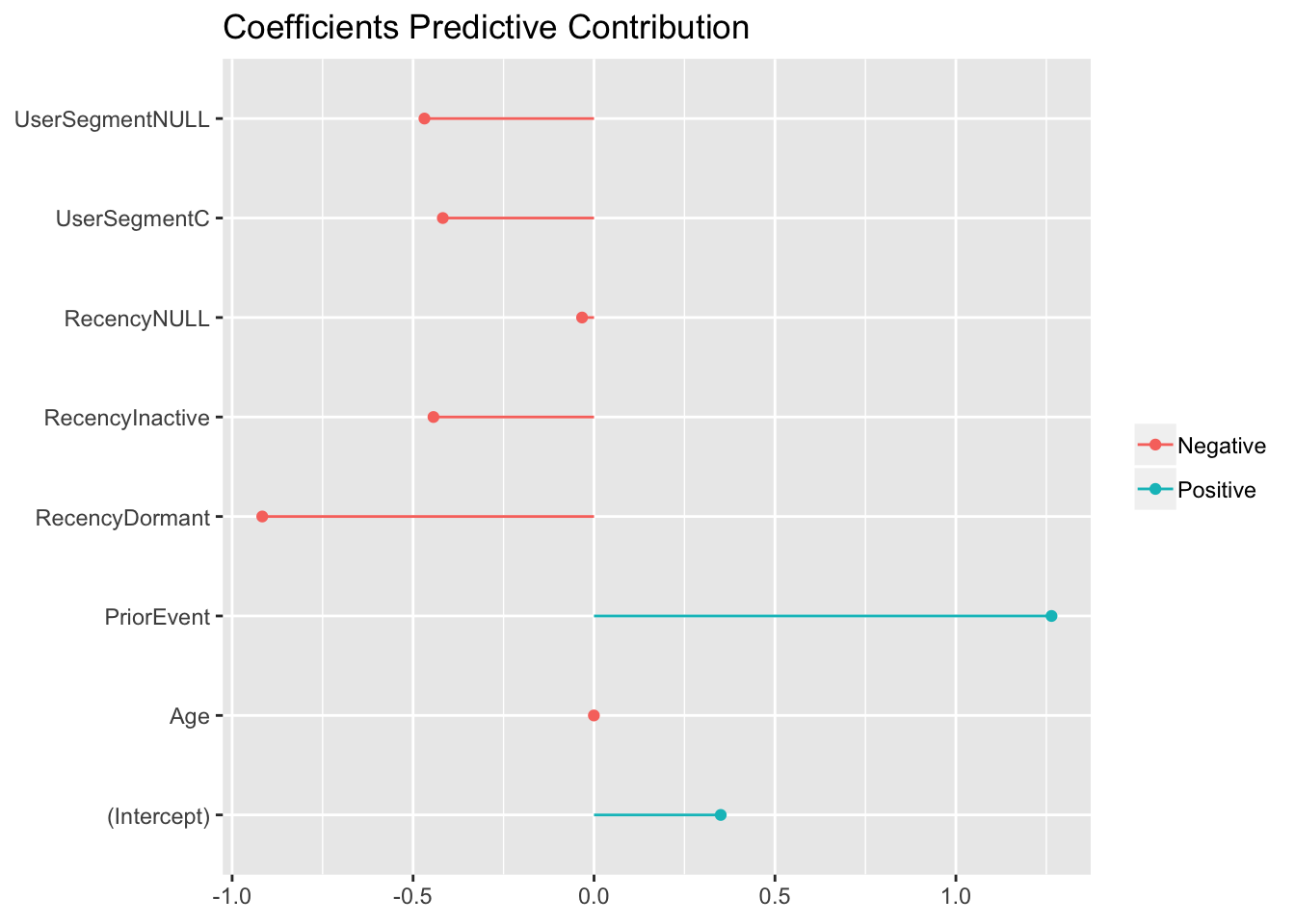
Finally, it is of a great interest to see which variables show strong predictive power and towards what behaviour. For instance, knowing the segment of a specific customer, would it help in recommending a particular product or would that push the user to the opposite direction? The graph below shows the predictive power of each variable as it was captured by the model.
## STORE THE LASSO LOGISTIC REGRESSION COEFFICIENTS
tmp_coef <- coef(cv, s = "lambda.min")   # COEF OF LAMBDA MIN
coef <- data.frame(name = tmp_coef@Dimnames[[1]][tmp_coef@i + 1], coefficient = tmp_coef@x)
b_coef <- coef[order(coef[,2]),]

## VISUALISE THE COEFFICIENTS
ggplot(b_coef, aes(y = b_coef[,2], x = b_coef[,1], color = if_else(sign(b_coef[,2]) > 0, "Positive", "Negative"))) +
  geom_point(stat = "identity") +
  geom_segment(aes(y = 0, x = b_coef[,1], yend = b_coef[,2], xend = b_coef[,1])) +
  coord_flip() +
  theme(axis.title.x = element_blank(), axis.title.y = element_blank(), legend.title = element_blank()) +
  ggtitle("Coefficients Predictive Contribution")
FUTURE DEVELOPMENT AND ENHANCEMENT
The proposed model is merely one of the main approaches in trying to predict customers behaviours and interests. For instance, when the data becomes large enough in terms of available variables, the suggested model may have some limitations. Moreover, it was stated by BGL that the data provided relates to a single, specific event/product. That means that the Logistic regression model needs to be run on a single product each time to make a recommendation. It is not difficult to understand that this is not an efficient way to make a recommendation, especially when there is a wide range of products or services available. Thus, an enhancement of the already proposed model would a Bayesian Logistic Regression model since prior knowledge is available or a hybrid model using Data Mining techniques along with Machine Learning. More specifically, the idea would suggest performing association rules to identify items that are frequently bought together. This can create some natural clusters where certain products can fall into. Finally, lasso regression could be run individually on these clusters to improve recommendations.
A very promising approach would also be to implement User-Item Collaborative Filtering. This approach gives suggestions to statements like: “Users who are similar to you also liked …”. It is worth mentioning that Collaborative Filtering can also be used as a hybrid model with Lasso Regression as described previously. Major recommendations systems (e.g. Netflix, Spotify, Amazon, Facebook, etc) are collaborative filtering models which are based on assumption that people like things similar to other things they like, and things that are liked by other people with similar taste.
Finally, a more complex approach would be functional clustering. The idea of functional clustering is that the Events as described in our dataset are not independent but connected. Therefore, the available data for every user can be transformed into a function (e.g. a line) and examined as such. Functional clustering is a really advanced approach that allows to further investigate user’s behaviours thoroughly. For instance, keeping in mind that every customer is represented as a function, various information can be extracted through the derivative of that function.
BROADER APPLICATIONS WITHIN COMPARETHEMARKET.COM
The aforementioned approaches were created with the purpose of recommending particular products to customers. Yet, these models can be used to answer a variety of challenging questions that BGL and comparethemarket.com are facing every day. Although we are certain to bring a decent recommendation system, a broader application of these models could assist in a better customer targeting or discovery of new products of interest for the users.
EXTRAS
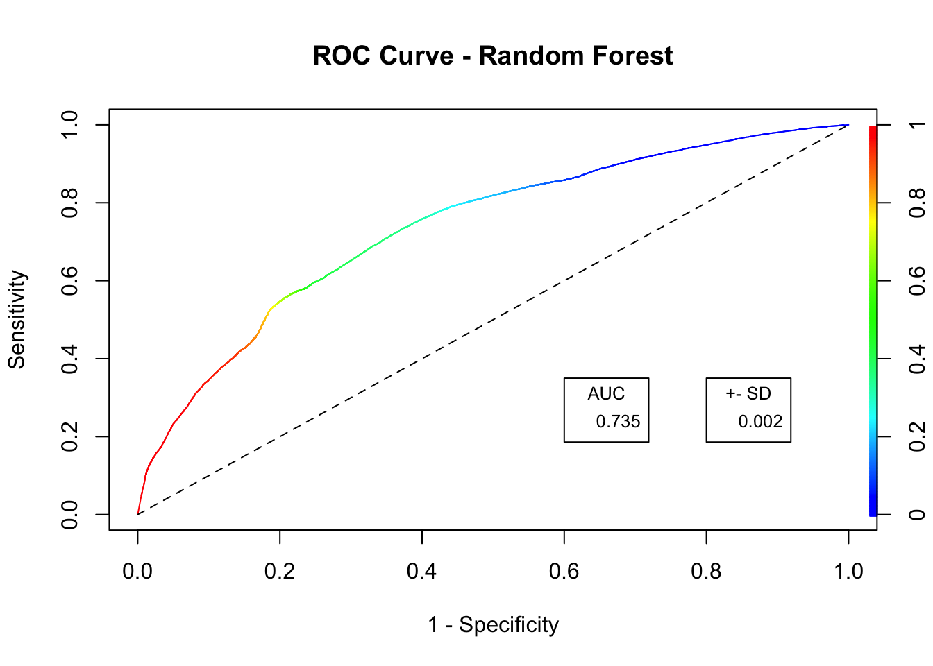
This section offers an attempt of different machine learning model for a product recommendation. The approach uses a quick implementation of the Random Forest algorithm. Note that Random Forest is a parametric model and thus, it is time-consuming to fully develop such a model.
## SET NUMBER OF REPETITIONS
n <- 10
## EMPTY CONFUSION MATRIX TO BE STORED FROM VARIOUS REPETITIONS
confusionRF <- data.frame(r1 = rep(0,n), r2 = rep(0,n), r3 = rep(0,n), r4 = rep(0,n))

## AUC VALUE EMPTY VECTOR TO STORE AUC VALUES FROM VARIOUS REPETITIONS
auc.totalRF <- vector(mode = "numeric", length = n)
OOB <- vector(mode = "numeric", length = n)

## RUN THE MODEL
for(i in 1:n){
  ## CREATE BALANCED DATASET BY UNDERSAMPLING THE MAJORITY CLASS
  event0 <- data[data$Event == 0,]
  event0 <- sample_n(event0, 30000, replace = FALSE)  ## FROM MAJORITY CLASS, TAKE A 30.000 SAMPLE

  event1 <- data[data$Event == 1,]    ## FROM MINORITY CLASS, TAKE ALL THE 30.000 INSTANCES
  balancedDataRF <- rbind(event0, event1)   ## CREATE THE BALANCED DATA

  ## TAKE THE DEISGN MATRIX
  designMatrixRF <- sparse.model.matrix(Event ~ .  , data = balancedDataRF[,-c(1)])[,-1]  ## REMOVE THE CUSTOMER ID AND THE INTERCEPT
  responseRF <- balancedDataRF$Event  ## STORE THE RESPONSE VARIABLE

  ## SPLIT IN TRAIN AND TEST SET
  ind <- sample(2, nrow(designMatrixRF), replace = TRUE, prob = c(0.8, 0.2))

  trainDataRF <- designMatrixRF[ind == 1,]
  responseTrainRF <- responseRF[ind == 1]
  dim(trainDataRF)

  testDataRF <- designMatrixRF[ind == 2,]
  responseTestRF <- responseRF[ind == 2]
  dim(testDataRF)

  ## CHECK FOR PROPORTION
  # FOR DESIGN TRAIN
  table(responseTrainRF)

  # FOR DESIGN TEST
  table(responseTestRF)

  ## RANDOM FORREST
  rf <- randomForest(x = as.matrix(trainDataRF), y = as.factor(responseTrainRF))
  rf

  OOB.error <- rf$err.rate[,1]
  OOB[i] <- OOB.error[length(OOB.error)]

  # tune(randomForest, train.x = as.matrix(train.data.rf), train.y = as.factor(response.x.rf))

  ## AUC VALUE
  prediction.rf <- as.vector(rf$votes[,2])
  pred.rf <- prediction(prediction.rf, ifelse(responseTrainRF == "1", 1, 0))
  auc.rf <- performance(pred.rf, "auc")
  auc.rf <- auc.rf@y.values[[1]]
  auc.totalRF[i] <- auc.rf

  # PREDICT ON UNSEEN DATA
  rf_pred <- predict(rf, testDataRF, cutoff = c(0.60, 0.40))

  # RESULTS
  confusionRF[i,] <- as.vector(table(as.factor(rf_pred), as.factor(responseTestRF)))

}

# VISUALIZATIONS
# plot(rforest)
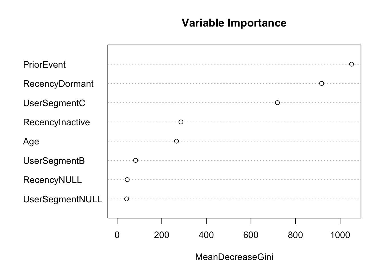
varImpPlot(rf, sort = TRUE, main = "Variable Importance")
## CREATE A FUNCTION TO CALCULATE THE AVERAGE ACCURACY, SPECIFICITY, SENSITIVITY OF THE VARIOUS REPETITIONS
res <- function(x) {
  x <- matrix(as.numeric(x), ncol = 2)
  accur <- (x[1,1]+x[2,2])/sum(x)
  sens <- x[2,2]/sum(x[,2])
  spec <- x[1,1]/sum(x[,1])
  out <- list(Accuracy = accur, Specificity = spec, Sensitivity = sens)
  out
}

## OBTAIN RESULTS
total.bal <-  apply(confusionRF, 1, FUN = res)

avg.spec.bal <-0
avg.acc.bal <-0
avg.sens.bal <- 0

acc.rf.total <- vector(mode = "numeric", length = n)
sens.rf.total <- vector(mode = "numeric", length = n)
spec.rf.total <- vector(mode = "numeric", length = n)

for(i in 1:n){
  avg.spec.bal = as.numeric(total.bal[[i]][2]) + avg.spec.bal
  spec.rf.total[i] <- as.numeric(total.bal[[i]][2])

  avg.acc.bal = as.numeric(total.bal[[i]][1]) + avg.acc.bal
  acc.rf.total[i] <- as.numeric(total.bal[[i]][1])

  avg.sens.bal = as.numeric(total.bal[[i]][3]) + avg.sens.bal
  sens.rf.total[i] <- as.numeric(total.bal[[i]][3])
}
## AVERAGE OOB ERROR
cat("The average Out Of Bag error for random forest is:", mean(OOB))

## AVERAGES
cat("The average accuracy of", n, "repetitions is:", round(avg.acc.bal/n, digits = 3))
cat("The average sensitivity of", n, "repetitions is:", round(avg.sens.bal/n, digits = 3))
cat("The average specificity of", n, "repetitions is:", round(avg.spec.bal/n, digits = 3))

## STANDARD DEVIATIONS
round(sd(acc.rf.total),3)
round(sd(sens.rf.total),3)
round(sd(spec.rf.total),3)

## ROC CURVE
prediction.rf <- as.vector(rf$votes[,2])
pred.rf <- prediction(prediction.rf, ifelse(responseTrainRF == "1", 1, 0))
roc.rf <- performance(pred.rf, "tpr", "fpr")

## AUC
auc.rf.avg <- round(mean(auc.totalRF),3)
auc.rf.sd <- round(sd(auc.totalRF),3)

plot(roc.rf, colorize = TRUE, ylab = "Sensitivity", xlab = "1 - Specificity", main = "ROC Curve - Random Forest")
lines(c(0,1), c(0,1), col = "black", lty = 2)
legend(.6, .35, auc.rf.avg, title = "AUC", cex = .8)
legend(.8, .35, auc.rf.sd, title = "+- SD", cex = .8)
