Hypothesis testing in statistics is a way for you to test the results of a survey or experiment to see if you have meaningful results. You’re basically testing whether your results are valid by figuring out the odds that your results have happened by chance. If your results may have happened by chance, the experiment won’t be repeatable and so has little use.
1. Introduction
As a data science geek, I constantly try to base a decision based on data and facts rather than gut feelings.
I see it more like a game - “What would data tell me?”

Sherlock Holmes would go against this game though as he defines gut feeling as the instinctual assumption based on four factors; observations, knowledge, experiences, and learned behaviours. For the sake of the game, I will bypass Sherlock because really…Who wants to argue with Sherlock?
Back to our game, it was one of these sunny days that I had decided to go for a stroll with a friend of mine discussing some new technologies that came out on a specific product that I had expressed my interest - no product placement here, ha!
As we were going back and forth with the pros and cons, I decided to let fate decide whether I should proceed with the purchase or not. And by fate, I mean data!
- “I am not sure I follow…” my friend told me.
- “Well my dearest friend, do you know the ‘Let the coin decide for you’ game?”
- “Yes - you throw a coin once and you call it heads or tails. Then, you take the respective decision based on the outcome” said my friend.
- “Exactly. The only difference is that I will throw the coin 7 times because I want to let fate reveal itself by going against the expected distribution of the coin toss”
The game was on!
To decide whether I should buy my beloved product, I would throw a coin 7 times.
If the outcome was extreme:
I would take it as fate telling me to buy the product.
Else
It would mean that I should follow my normal path without proceeding with the purchase.
2. Terminology
Before we crack on with the problem, it would be a good idea to include some useful terminology that will help us make our decision.
2.1 Parameter
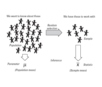
A Parameter is a summary description of a measure of interest that refers to the population parameter. The parameter never changes because everyone/everything was included in the survey to derive the parameter. In other words, it is the ground-truth value that we usually want to estimate from a sample.
Examples: Mean (μ), Variance (σ²), Proportion (π)
2.2 Statistic
A Statistic is, in a sense, opposite from the parameter and that is because a statistic refers to a small part of the population, i.e. a sample of the population.
In real-world, it is not feasible to get a complete picture of a population. Therefore, we draw a sample out of the population to estimate the population parameter. The summary description of the sample is called (sample) statistics.
Examples: Sample mean (x̄), Sample Variance (S²), Sample proportion (p)
2.3 Sample Distribution
A sampling distribution is the probability distribution of a sample statistic that is formed when samples of size n are repeatedly taken from a population. If the sample statistic is the sample mean, then the distribution is called the sampling distribution of sample means.
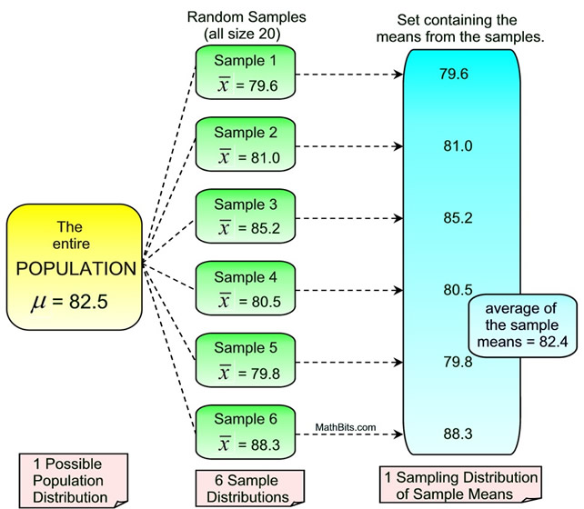
In general, we would expect the sampling the mean of the sampling distribution to be approximately equivalent to the population mean i.e. E(x̄) = μ
2.4 Standard Error
The standard error quantifies the variation in the means from multiple sets of measurements.
A confusion that usually arises in regards to the Standard Error is what is the difference with the standard deviation. And understandably given that both are measures of spread. Frankly, these two terms are equal to one main difference.
While the standard error uses statistics (sample data) standard deviation use parameters (population data).
In a nutshell, the standard error tells you how far your sample statistic (like the sample mean) deviates from the actual population mean. The larger your sample size, the smaller the standard error (SE). In other words, the larger your sample size, the closer your sample mean is to the actual population mean.
If this still does not make sense, please make sure to check this video from StatQuest with some useful visualisation to capture the difference between standard error and standard deviation
2.5 Type I & Type II error
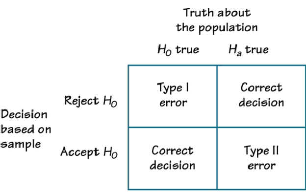
When we use the power of statistics, we are interested in making wise decisions based on data. We want to know if our action is well justified by substantial evidence - the evidence we observed. However, even in the presence of data, it is easy to be tricked and take a false decision due to an outcome that was observed by chance and not by an actual effect that is present in our population. These errors are known as the Type I & Type II error.
-
Type I error
Type I error occurs when an effect was captured by chance and we reject the null hypothesis when the null hypothesis is true. -
Type II error
Type II error occurs when the null hypothesis is not rejected when it is, in fact, false.
i.e. an effect is present but we failed to detect it.
3. Hypothesis Testing
Conducting a hypothesis testing follows a specific methodology as shown in the image below
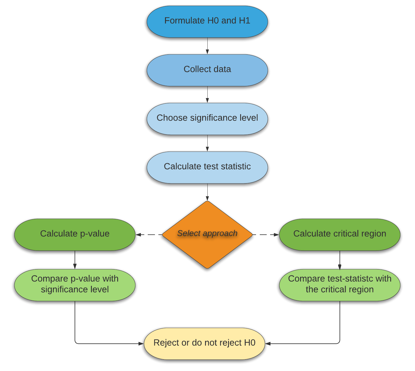
We are going to follow that exact framework to conduct our experiment. And so, without further due, my friend and I were ready to collect the data and see what fate has to say.
3.1 Formulate Hypothesis
We take out a (fare?) coin from our pockets and we are ready to throw it. We randomly assigned success as landing Heads and if the (extreme) result was in favour of Heads, I would proceed with the purchase.
The hypothesis formulation is quite straightforward:
\[H_{0}: \pi = 0.5 \leftrightarrow H_{1}: \pi > 0.5\]That means that I would expect the true proportion of landing Heads to be 0.5 (i.e. 50%) as opposed to the alternative saying that is larger.
3.2 Collect Data
Recall, that I would throw the coin 7 times - and 7 times I did!
The outcome was the following:
- Head (H): 6 times out of 7
- Tails (T): 1 time out of 7.
We can easily understand that the sample proportion equals p = 0.86
One interesting thing to note here is that under the assumption of the null hypothesis, sample proportions $ \hat{p} $ should follow an approximately normal distribution.
This is established thanks to the Central-Limit theorem which states that if you have a population with mean μ and standard deviation σ and take sufficiently large random samples from the population with replacement, then the distribution of the sample means will be approximately normally distributed.
Therefore, I know that, thanks to CLT, my sampling distribution is:
\[\hat{p} \sim \mathcal{N}(\mu = p = 0.5, \sigma = SE = \sqrt{\frac{p(1-p)}{n}} = 0.19)\]Note: For the central limit theorem to stand, some conditions have to be met. For the sake of my game, I assume that they stand even though I am aware that this is not true (e.g. according to CLT, np >= 10 which does not hold in our case).
Excellent!
3.3 Inference
To make up my mind now, all I want to know is how extreme my observation is (i.e. the outcome of my coin tosses) under the null hypothesis. In other words, how ridiculous do my observations make my null hypothesis look; If they make it look more ridiculous than a specific tolerance level, then I can conclude that I have strong evidence to reject my null hypothesis.
There are two approaches we can follow and we will discuss both of them. We are also going to include some additional terminology along the way such as the tolerance threshold I mentioned - spoiler alert; this is the significance level (α).
Significance Level
The probability of making a Type-I error is denoted by alpha (α). Alpha is the maximum probability that we have a Type-I error. For a 95% confidence level, the value of alpha is 0.05 (i.e. 5%). This means that there is a 5% probability that we will reject a true null hypothesis.
The significance levels during hypothesis testing is to help determine which hypothesis the data support. It’s the threshold that measures the strength of the evidence that must be present in the sample before we can reject the null hypothesis and conclude that the effect is statistically significant.
For the sake of our example, we will use a confidence level equal to 0.05. (i.e. α = 0.05)
P-Value
In statistical testing, the p-value is the probability of obtaining test results at least as extreme as the results observed, under the assumption that the null hypothesis is correct.
It measures how compatible your data are with the null hypothesis. How likely the effect observed in your sample data if the null hypothesis is true?
3.3.1 Approach - Critical Region
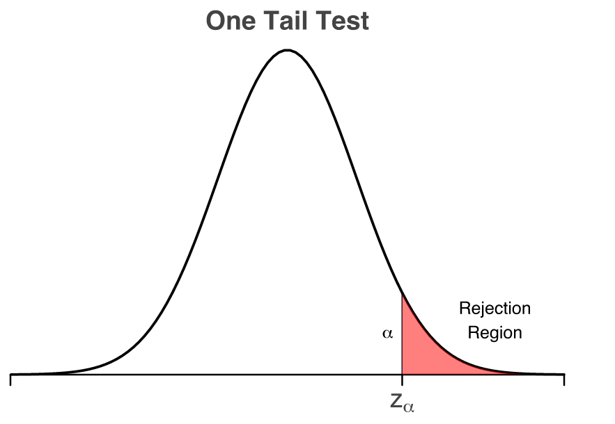
For the critical region approach, we are only interested to capture the z-score that will mark the “borbers” of the critical region and compare it with our z-score. By having a significance level of 0.05, we want to find the $z_{α}$ value as shown below
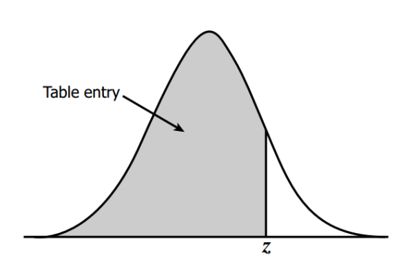
We can use the z-table to find the corresponding z-score. We are interested to find the z-score value from which point on, the shaded area (i.e. the probability) is 0.05 (i.e. 5%). Hence, we are interested for the shaded area that gives as a probability of 1 - α = 1 - 0.05 = 0.95.
The picture below might be able to show a nice visual if that was not clear.
Using the z-table, we find that the z-score that marks the critical region is 1.645. In other words, $z_{α}$ = 1.645
Now, we need to calculate the z-score of our sample and compare it with the z-score of the critical region to know whether falls within the critical region or not.
For the z-score, we use the following formula:
\[z = \frac{\hat{p} - p}{SE}\]Doing the maths, $ z = \frac{\hat{p} - p}{SE} = \frac{0.86 - 0.5}{0.19} = $ 1.89
3.3.2 Approach - p-value
We said before that a p-value is the probability of observing a result at least as extreme as the result observed. In other words, we want to know that if we live in the world that the null hypothesis is true, how extreme or how probable my observation of 6 heads and 1 tail would be.
This is what the p-value will tell me.
To calculate the p-value, I need to find the z-score following the formula mentioned above.
To recall, $ z = \frac{\hat{p} - p}{SE} = \frac{0.86 - 0.5}{0.19} = $ 1.89
Given that we have the z-value, we use the z-table probabilities to find our p-value
p-value $ = P(\hat{p} > 1.89) = 1 - P(Z < 1.89) = 1 - 0.9706 = 0.0294$
Our p-value is 0.0294.
4. Decision Making
With all of these calculations, we may have forgotten why we were doing the hypothesis testing in the first place - let me refresh your memory!
I was interested to know if the coin was fare (i.e. not buy my beloved product) or if the coin was not fare (i.e. I would interpret that as fate telling me to buy the product by making me observe an extreme outcome).
Let’s go ahead and take our decision for our two approaches - exciting stuff!
4.2 Critical Region
For the critical region approach, we calculated that our z-score = 1.89 whereas the z-score of the critical region (denoted as $ z_{α} $) is 1.645.
Given than 1.645 < 1.89 (hence our z-score falls within the critical region), we conclude that we reject the null hypothesis and that we have significant evidence to say that I can proceed and buy the product - yeah!
4.3 P-Value
We can expect that the p-value approach will yield the same result but for sanity’s sake, let’s interpret the results as well.
For a significance level of 0.05 and a p-value of 0.0294, we can see that 0.0294 < 0.05. As a result, we conclude that we reject the null hypothesis and that we have significant evidence to say that I can proceed and buy the product - yeah! x2.
5. Conclusion
I hope you have enjoyed this read as much as I enjoyed writing it!
The purpose of this post was to introduce a playful way of using hypothesis testing without going through the strict assumptions under the central limit theorem. Nevertheless, the mindset and methodology of conducting a hypothesis test can be used in any framework to make a wise decision under uncertainty.
Cheers!
References
Everything you need to know about hypothesis testing

