AdaBoost (Adaptive Boosting) is a popular boosting algorithm that combines multiple weak classifiers to create a strong classifier.
The algorithm works by iteratively adjusting the weights of the training instances and focusing more on the misclassified instances in each iteration using a weighted sampled distribution.

AdaBoost

Assume we have some data $\{(x_{i}, y_{i} )\}_{i=1}^{n}$ with $y_{i}$ being a binary column $\in {-1, 1}$.

Initialize the weights of the training instances:

$w_i^{(1)} = \frac{1}{n}$ for $i = 1, \dots, n$
For each iteration from 1 to $t$:

a. Train a decision tree classifier $h_t(x_i)$ on the training data with weights $w_i^{(t)}$.

💡 The Gini index is being used to decide which feature will produce the best split to create the stump tree. The Gini index formula is $G = \sum_{i=1}^J p_i (1 - p_i)$ where $J$ is the number of classes, and $p_i$ is the proportion of instances with class $i$ in the current node.

Note: Each weak classifier should be trained on a random subset of the total training set. AdaBoost assigns a “weight” (i.e. weighted sampling method) to each training example, which determines the probability that each example should appear in the training set.

💡 AdaBoost makes super small decision trees (i.e. stumps).

b. Calculate the error of the weak classifier:

$\epsilon_t = \sum_{i=1}^n w_i^{(t)} I(y_i \neq h_t(x_i))$

💡 The error term above basically sums up the weights of the misclassified examples which is being used in the formula c. to calculate the weight of the classifier $h_{t}(x_{i})$.

c. Calculate the weight of the weak classifier $h_t(x)$:

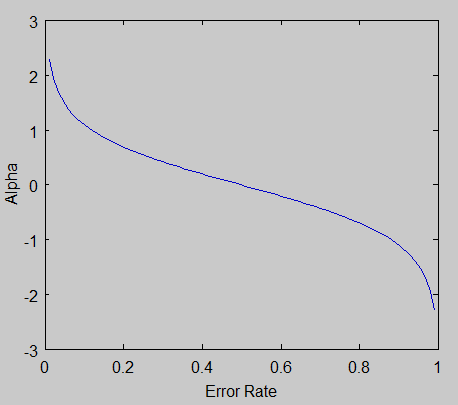
$\alpha_t = \frac{1}{2} \ln(\frac{1 - \epsilon_t}{\epsilon_t})$

💡 This is just a straightforward calculation replacing $\epsilon_{t}$ from formula b. above. Here is the graph of $\alpha$ looks for different error rates $ln(\frac{1 - \epsilon}{\epsilon})$
💡 The intuition of the graph is three-fold:
1. The classifier weight grows exponentially as the error approaches 0. Better classifiers are given exponentially more weight.
2. The classifier weight is zero if the error rate is 0.5. A classifier with 50% accuracy is no better than random guessing, so we ignore it.
3. The classifier weight grows exponentially negative as the error approaches 1. We give a negative weight to classifiers with worse than 50% accuracy. “Whatever that classifier says, do the opposite!”.
d. Update the weights of the training instances:

$w_i^{(t+1)} = \frac{w_i^{(t)} e^{-\alpha_t y_i h_t(x_i)}}{Z_{t}}$
, where $Z_t$ is a normalization factor → $Z_t = \sum_{i=1}^n w_i^{(t)} e^{-\alpha_t y_i h_t(x_i)}$
💡 In the original paper, the weights $w_{i}$ are described as a distribution. To make it a distribution, all of these probabilities should add up to 1. To ensure this, we normalize the weights by dividing each of them by the sum of all the weights, $Z_t$. This just means that each weight $w_{i}$ represents the probability that training example $i$ will be selected as part of the training set.

Also, $y_i$ is the correct output for the training example $i$, and $h_t(x_i)$ is the predicted output by classifier $t$ on this training example.
1. If the predicted and actual output agrees -> $y*h(x)$ will always be +1 (either $1*1$ or $(-1)* (-1)$).
2. If the predicted and actual output disagrees -> $y * h(x)$ will be negative.
Output the final strong classifier:

$H(x) = \text{sign}\left(\sum_{t=1}^T \alpha_t h_t(x)\right)$
💡 The final classifier consists of $T$ weak classifiers:
1. $h_t(x)$ is the output of weak classifier $t$.
  Note: In the paper, the outputs are limited to -1 or +1.
2. $\alpha_t$ is the weight applied to classifier $t$ as determined by AdaBoost in step c.
As a result, the final output is just a linear combination of all of the weak classifiers, and then we make our final decision simply by looking at the sign of this sum.

AdaBoost for the win!

Adaptive Boosting - The first of its kind!

AdaBoost for the win!

Adaptive Boosting - The first of its kind!

AdaBoost